Help

Gene expression is read from tab delimited files with the following format:
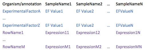
Here you can find several examples.
NOTES:
-
•organism can be any text defining the organism of the experiment, but we recommend to use scientific names (e.g. Homo sapiens)
-
•annotation can be any text describing gene identifiers, but in order to retrieve functional annotation, gene names, etc. BicOverlapper would need one of the following (otherwise, these options would be disabled):
-
-A BioConductor annotation package database name (those with .db extension), such as hgu133plus2.db
-
-biomaRt.xxx where xxx is the type of identifier as BioMart describes them on its BioConductor package. For example: biomaRt.external_gene_id
-
•experimental factors (EF) can be any text that refer to conditions that are tested in the experiment, such as Tissue, Disease State, Sex, Treatment, Time, etc.
-
•experimental factor values (EFV) can be any text that refer to especific instances of the EF, such as Prostate, Healthy, Female, Non-treated, 2 hours, etc. NOTE: in order to perform some types of analysis (such as GSEA or differential expression), two or more replicates of each EFV are required.
-
•row names must be unique probe/gene ids of the type provided in annotation
-
•expresion levels are real numbers (decimal separator must be a point). Although we generally refer to expression levels, they may be any numerical measure.
Gene expression Data
You can directly download experiments from GEO or ArrayExpress into BicOverlapper.
GEO:
GEO experiments are downloaded via BioConductor package GEOquery. GSExxx accession number is required, and only the processed data are loaded.
The interface also permits to perform a log transform on the data.
The experiment is stored as a BicOverlapper gene expression data file.
NOTE: GEOquery retrieves experimental factors in a single field, so you might want to edit the
corresponding lines of the file in order to properly identify them.
ArrayExpress
ArrayExpress experiments are downloaded via ArrayExpress BioConductor package. Any accession number can be used, although multiarray chips and several other experiments might not be available to download via this package. Usually, MEXP and TABM experiments can be downloaded, but other types are often unavailable.
NOTE: Experiment download is time consuming and there are multiple format issues that might break the process. We recommend to download small experiments (up to 10 samples) with single chip platforms.
Download experiments
BicOverlapper relies on R/BioConductor to work. If you don’t have the required package for any process, BicOverlapper will tell you to install it from R.
These are the most important packages used by BicOverlapper:
-
•biclust, isa2: These CRAN-R packages are used to perform biclustering analysis on gene expression.
-
•limma: this package is necessary to perform differential expression searches based on replicates and statistical significance.
-
•GSEAlm: required in order to perform GSEA enrichment analysis
-
•ArrayExpress, GEOquery: These packages are used to download gene expression experiments directly from the corresponding databases.
-
•affy: package required to normalize raw data in the case RMA is selected when downloading ArrayExpress experiments
-
•GO.db, annotate: These packages are used in order to manipulate GO annotations. GOstats: This package is used to perform hypergeometric GO significance tests.
-
•annotation packages: they are used in the case of microarray platforms with an available BioConductor annotation package. For example, if the data come from Affymetrix Yeast Genome S98 chips, then ygs98.db package should be installed.
-
•biomaRt: if row ids correspond to any gene id supported by biomaRt annotation package, this is required in order to retrieve gene annotations and synonyms. You should use as annotation in the matrix file biomaRt.xxx where xxx is the type of BioMart identifier (e.g. biomaRt.external_gene_id)
-
•MASS: used to save matrices after merging columns
R/BioConductor
BicOverlapper allows several types of analysis:
-
•Select profiles: the most simple type of analysis, selects all the genes with expression between certain limits, in terms of standard deviations, for a given Group of conditions, and, optionally, against another Group.
-
•Differential expression: based on limma Bioconductor package, it searches for genes differentially expressed on Group 1 conditions respect to Group 2 conditions. Note that Groups 1 and 2 are experimental factor values, and they must have more than one replicate in order to perform this analysis.
Multiple group differential analyses can be done at once by selecting the name of the experimental factor instead of one of its values.
-
•GSEA: Gene Set Enrichment Analysis searches for the GO or KEGG terms that are enriched on the experiment, again respect to two groups of experimental factors.
-
•Biclustering: There are several biclustering algorithms available. Each one has a different set of parameters. Briefly:
-
-Bimax searches for elements with very high expression levels
-
-Plaid model searches for elements that vary in the same way (shift factor)
-
-ISA is the Iterative Search Algorithm as in isa2 Bioconductor package
-
-xMotifs searches for elements that conserve expression between certain ranges
-
-Cheng & Church searches for elements that vary in the same way (shift factor)
-
•Correlation network: This method builds a network using as nodes the genes that present high variance among samples and links them if there are small profile distances among them. The result can be saved in GML format.
NOTE: when using these data mining methods, it is very important to do a correct parametrization. Too loose parameters usually derive in long computation times and very cluttered visualizations, and may hang the tool. In the case of biclustering, this is especially important, and a post-filtering step can be applied to remove redundant groups. In case of doubt, it is desirable to start with very stringent parameters and then iterate towards less restrictive ones until patterns arise.
Analysis
Bicoverlapper has several visualizations for biological data:
-
•Parallel Coordinates: represent expression profiles as lines with a height proportional to the expression level at each condition (vertical axes). On the background, boxplots with the distribution of values for each condition is displayed. Some interaction options:
-
-Drag the scrolls at the tips of the axes to select elements between the dragged threshold. If the number of elements is large a blue shade is drawn, otherwise each element is drawn as a line.
-
-Ctrl+drag to filter only by the current scroll (ignoring any other ones)
-
-Remember that you can use shortcuts Ctrl-z, Ctrl-y, Ctrl-0 (see below)
-
•Heatmap: classical representation of expression profiles, on a blue-white-red scale for low-average-high expression. The heatmap is only displayed when a small number of elements has been selected. There are some interaction options:
-
-Mouse drag to select a subgroup of genes
-
-Alt+click a gene: opens the Entrez Gene webpage entry
-
-Ctrl+click a gene: searches for genes with a similar profile
-
-Right-click to show a configuration panel for color scale, etc.
-
•Overlapper: Venn-like representation of groups. Each group is represented as a ‘bubble’ with elements (genes or conditions) inside. Disjoint zones are represented as circles or piecharts if shared by two or more groups. Bubble size is proportional to the number of elements in the group. Position and shape depend on a force-directed layout that keeps close elements in the same groups and separate elements in different ones (more info on this paper). Some interaction options:
-
-Mouse over to highlight groups or elements
-
-Click to select groups or single elements or zones
-
-Draw a line for area selection
-
-Drag the overview box to navigate through the visualization space
-
-Drag in the main view to zoom in/out
-
-Press ‘u’ to switch between summarized and complete views
-
-Press ‘p’ to pause/resume force-directed movement
-
-Press ‘n’, ’t’, ’l’, ’a’, ’h’ to hide/show nodes, titles, labels, arcs or hulls, respectively
-
-Right-click on a gene to get a summary description
-
•Bubble map: PCA representation of groups. Simpler than Overlapper, it is recommended to visualize large numbers of groups, but intersections between groups are harder to identify. BicOverlapper will automatically select Bubble map or Overlapper depending on the number and complexity of the groups found.
-
•Network: Force-directed network. If more than 200 genes are selected, the network will be possibly too cluttered to see patterns.
-
-Mouse wheel to zoom
-
-Click and drag the background to pan
-
-Click to select elements or alt-click to add to the selection
-
-Right-click the background to fit into screen
-
•Word cloud: Functional terms are drawn as a tag cloud. Tags are alphabetically sorted and the size correspond to the number of selected elements that are annotated with each term, which is also shown in parenthesis.
NOTE: when using these data mining methods, it is very important to do a correct parametrization. Too loose parameters usually derive in long computation times and very cluttered visualizations, and may hang the tool. In the case of biclustering, this is especially important, and a post-filtering step can be applied to remove redundant groups. In case of doubt, it is desirable to start with very stringent parameters and then iterate towards less restrictive ones until patterns arise.
Visualization
Bicoverlapper implements some key shortcuts to access menu options and others.
-
•Undo selection: Ctrl+z
-
•Redo selection: Ctrl+y
-
•Reset selection: Ctrl+0
-
•Sort columns: Ctrl+s
-
•Change labels: Ctrl+l
-
•Search text: Ctrl+f
-
•Export figure: Ctrl+p
Shortcuts
If you have your own grouping method, you can visualize it with Overlapper if you format its output into our .bic format:
Number_of_groups
Free text description line
Name_of_bicluster_1 : number_of_rows number_of_cols
id_row id_row ... id_row
id_col id_col ... id_col
...
Name_of_bicluster_N : number_of_rows number_of_cols
id_row id_row ... id_row
id_col id_col ... id_col
Here you can find some examples.
Some notes:
-
•Name_of_bicluster_X and Free text description line can contain spaces, but not tabs
-
•Number_of_groups, number_of_rows and number_of_cols must be integers.
-
•number_of_cols can be 0. In that case, leave an empty line instead of id_col id_col ... id_col
-
•id_col and id_row must correspond to rowNames and sampleNames in the Expression Data (see above) if you want them to be linked in the visualization.
-
•number_of_rows, number_of_cols and ids must be tab separated.
Group Data
Data can be exported by giving a file path previously to its generation, on the following cases:
-
•Expression data downloaded from ArrayExpress or GEO can be saved if a path is selected at the corresponding download panels, as tab delimited files with the format described above (Expression Data section)
-
•Group data can be saved if a path is selected at the different analysis panels that generate groups, as a tab delimited file with the format described above (Group Data section)
-
•Network data can be saved if a path is selected at the ‘Analysis/Compute Network...’ option panel, as a GraphML file.
Selected genes can be exported as a text list at any time with the option ‘File/Export Selection’.
Figures can be exported at any time with the menu option ‘File/Export Figure’ or with Ctrl+p, on PNG or EPS formats. Figures are saved at a size higher than the actual visualization in order to improve resolution. NOTE: although functional, this is by now still an option under development and may change in the future.
Exporting data